The bioSDP Tutorial
This tutorial describes the use of the bioSDP Toolbox for Matlab along the lines of a simple application example.
The core functionality of the toolbox is
- approximation of feasible steady state sets for a biochemical network model, given a parametric uncertainty;
- approximation of the set of parameters in a biochemical network model which is consistent with uncertain measurement data;
- visualization of the resulting uncertainty sets.
Background
The main goal of system biology is a quantitative description of cellular processes and the understanding of those. Unfortunately, achieving this aim is rather difficult, as models of biological systems are subject to a significant degree of uncertainty. This uncertainty arises from limited knowledge about the system, mostly due to limitations in the experimental technology, and/or large variations in environmental and internal boundary conditions. The uncertainties become manifest in a only partially known interaction structure and unknown parameter values, and most models of biochemical networks show large parametric and/or structural uncertainties. It is a major computational problem to draw dedicated conclusions about diverse system properties under such uncertainty.
The bioSDP toolbox provides methods to study the variation in steady states of a network under parametric uncertainty. As an additional feature, it allows to upper-bound the size of the remaining parametric uncertainty from noise corrupted measurement data. In contrast to other computational methods to deal with these tasks, the methods employed in this toolbox provide guaranteed upper bounds on the uncertainties. This allows to derive guaranteed predictions about important system properties given only limited information about the process.
Steady state uncertainty analysis
Background
In many situations only the long term behavior of a biological process is relevant. Reasons for this may be that
- the dynamics of a process are very fast, or that
- it does not matter at which time instance but just that a particular signaling event occurs.
Well known example for this are stem cell differentiation after the stimulus with a differentiation signal, and programmed cell death (apoptosis) of tumor cells after the stimulus with an anti-cancer drug. There, the only thing we are interested in is whether a cell differentiates/dies, or not. Also from a theoretical point of view steady states play a crucial role, as they determine the asymptotic properties of systems.
The uncertainty analysis of the steady state can reveal important information. The most obvious is the strength of the dependency of the steady state concentration of particular species on particular uncertain parameters. This may help to understand which parameters are highly relevant and which states are inert to even large changes in parameter values.
Running example
The usage of the bioSDP toolbox will be illustrated in this tutorial with a simple example network, namely a simplified insulin signaling pathway. The network is given by the following reactions:
v1: IR -> IRP, rate = k1basal*IR + k1*insulin*IR
v2: IRP -> IRi, rate = k2*IRP
v3: IRi -> IR, rate = kR*IRi
v4: IRS -> IRSP, rate = k3*IRP*IRS
v5: IRSP -> IRS, rate = km3*IRSP
While it is not strictly necessary to remove conservation relations from the network before doing the analysis, it is suggested to do so, since it reduces the number of uncertain variables, which is one of the key influential factors for the computation time. In the example of the insulin pathway, we have the conservation relations:
IR + IRP + IRi = IRtot
IRS + IRSP = IRStot
Using the conservation relations to replace IRi and IRS in the above reaction rates, we retain the three state variables IR, IRP, and IRSP.
Problem setup
The system to be analyzed must belong to the class of nonlinear ordinary differential equations (ODEs):
xdot = f(x,p),
with state vector x and parameter vector p.
In the current implementation of the toolbox, the vector field f must be polynomial in the elements of x and p. Network models with Michaelis-Menten or Hill reaction rates can be studied either by multiplying the equations with the denominator, or by introducing additional variables.
In steady state uncertainty analysis, the goal is to find an outer approximation of the set of all feasible steady states of the network model, given that parameters are allowed to vary within specified regions of the parameter space. These are all vectors x for which there exist a parameter vector p within the specified uncertainty such that f(x,p) = 0 hold.
To set up the steady state uncertainty problem for the bioSDP toolbox, we first have to specify the state vector x, parameter vector p, system equations f. This information is collected in a Matlab structure which is called system in this tutorial. The following Matlab code defines the uncertain variables as symbols and sets up the system structure:
>> syms IR IRP IRS
>> syms k1 k1basal k2 kR k3 km3 insulin
>> system.x = [IR; IRP; IRSP];
>> system.p = [k1; k1basal; k2; kR; k3; km3; insulin];
>> IRtot = 10;
>> IRStot = 10;
>> system.oderhs =  [ - k1*IR*insulin - k1basal*IR + kR*(IRtot-IR-IRP);
                      + k1*IR*insulin + k1basal*IR - k2*IRP;
                      - km3*IRSP + k3*IRP*(IRStot-IRSP) ];
Furthermore, the uncertainty in the parameter vector p as well as an initial outer bound on the state variables have to be specified. This is done within a Matlab structure which is called uncertainty in this tutorial:
>> uncertainty.pmin = 0.5*[0.05; 10e-6; 1.0; 0.5; 1.0; 30; 1.0];
>> uncertainty.pmax = 2.0*[0.05; 10e-6; 1.0; 0.5; 1.0; 30; 1.0];
>> uncertainty.xmin = [0; 0; 0];
>> uncertainty.xmax = [IRtot; IRtot; IRStot];
Note that the initial outer bound for the state variables is directly derived from the conservation relations in this example.
Running the solver
The main bioSDP Toolbox routine for steady state uncertainty analysis is the function stationary_uncertainty.m. This routine takes the problem setup specified in the variables system and uncertainty, and computes an outer approximation of the set of feasible steady states. The behaviour of the uncertainty analysis function is further controlled by several options, which are passed as a structure variable called options in this tutorial.
A required option is options.set_exclusion.method, which specifies how regions in state space are removed from the feasible set. The default choice is 'box shrinkage', which just tries to reduce the size of the initial box as far as possible. A method which allows to obtain a more refined uncertainty set is 'bisection', in which the uncertainty set is computed by bisection. However, the bisection method is only recommended for state spaces up to dimension three due to significantly increased computational effort in higher dimensions. For the tutorial, we nevertheless choose the 'bisection' method since its results provide more visualization options:
>> options.set_exclusion.method = {'bisection'};
The steady state uncertainty analysis function is then called as:
>> [sdpresult, sdpproblem] = stationary_uncertainty(system, uncertainty, options);
Several other options concerning mainly the numerics of the uncertainty analysis algorithm are available, for example the termination criteria for the approximation. Further details are described in the inline documentation for the steady state uncertainty analysis, which can be accessed from the Matlab command line:
>> help stationary_uncertainty
Sampling feasible steady states
In order to evaluate the tightness of the computed approximation to the steady state uncertainty set, the bioSDP toolbox provides the routine sample_steady_states.m to sample feasible steady states under the given parametric uncertainty:
>> [samples] = sample_steady_states(system, uncertainty)
The behaviour of the sample_steady_states method can be controlled by further options, as detailed in the inline documentation.
Visualization of the results
To obtain a quick glimpse of the steady state uncertainty sets, the bioSDP Toolbox features plotting these sets as parallel coordinates. This gives a good visual overview even for high-dimensional state spaces. Another, more detailed, plot type are 2D or 3D box plots of the resulting uncertainty sets. However, this option is not available if the dimension of the state space is higher than three.
To plot the uncertainty sets, the Matlab function visualize_uncertainty is provided. Its arguments are the system description and the uncertainty structure which resulted from the previous analysis:
>> visualize_uncertainty(sdpresult);
This function call produces two plots: a plot of the uncertainty intervals in each state variable, and a three-dimensional plot where boxes that potentially contain steady states are shown in blue:
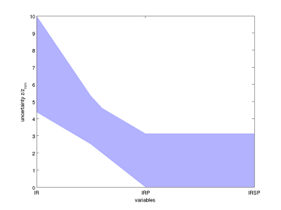
Steady state uncertainty sets plotted in parallel coordinates.
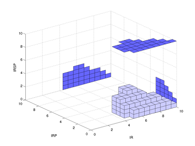
Steady state uncertainty sets plotted as 3D boxes.
In the parallel coordinates plot, the thinning waist between IR and IRP indicates a slight negative correlation between these two variables. This correlation is also seen more explicitly in the three-dimensional box plot.
A visual evaluation of the tightness of the computed outer approximation is obtained by comparison with the sampled steady states, which are also passed to the visualization routine:
>> visualize_uncertainty(sdpresult, samples);
Here, the sampled steady states are plotted in parallel coordinates, together with the computed outer approximation which is guaranteed to contain all possible steady states under the given parametric uncertainty.
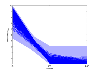
Steady state uncertainty sets plotted in parallel coordinates. Blue lines represent sampled steady states.
Parameter estimation
Background
The main idea behind set-based methods is to analyze regions in parameter space instead of single points. This can be done using different approaches. The most well known are interval analysis methods. In the bioSDP Toolbox, methods from convex optimization are applied. The advantage of studying sets in parameter space, instead of single points is, that guarantees can be obtained. It may for instance be possible to show that a certain set in parameter space does not contain parameters which are consistent with the measurement data.
With this motivation, the bioSDP toolbox provides methods to compute an outer approximation to the set of consistent parameters, i.e. the set of parameters for which the model behaviour would fit to given uncertain measurement data. A particular application of this approach is model falsification: if the set of consistent parameters is empty, then there are no parameters for which the model can reproduce the measurement data, even taking uncertainty in the data into account.
Running example
The set based parameter estimation is illustrated in this tutorial for a simplistic network, a simple reversible modification of a single protein. The network is made up by the following two reactions:
modify: P -> Pm, rate = km*P
demodify: Pm -> P, rate = kd*Pm
Thereby, P is the unmodified protein , and Pm is the modified protein. km and kd are the parameters to be estimated based on uncertain measurements of P. The total concentration of the protein in the cell is known:
P + Pm = 1.0
Measurements have been performed at 5 time points in the course of an experiment, and holds lower and upper bounds on the concentration of P at these time points. These bounds are as shown in the following table.
| Lower bound | Upper bound |
|---|---|
| 0.00 | 0.10 |
| 0.44 | 0.54 |
| 0.57 | 0.67 |
| 0.60 | 0.70 |
| 0.56 | 0.66 |
For the parameters km and kd, we assume that a priori bounds are previously known, with 0 as a lower bound and 10 as an upper bound on each individual parameter.
Problem setup
Set based parameter estimation can be done with the bioSDP Toolbox for models described by a difference equation of the form:
x(k+1) = F(x(k),p)
  y(k) = H(x(k),p),
where x is the n-dimensional state vector of the system, p is the q-dimensional parameter vector, and y is the m-dimensional output available for measurement at each time point k. The vector field F as well as the output function H have to be polynomials in the state variables and the parameters.
As in the steady state uncertainty analysis, the bioSDP Toolbox uses a Matlab structure variable system to hold all information about the system for which set based parameter estimation should be done. The first pieces of required information is the parameter vectors, defined by the following Matlab code:
>>> syms km kd
>>> system.p = [km; kd];
The vector field F is usually not directly constructed by the user: difference equations are not very common in systems biology---most models are constructed as ordinary differential equations. Therefore, the bioSDP Toolbox offers methods to construct the required information about the dynamics from the discretization of a differential equation model. We first define the right hand side of the differential equation describing the protein modification network as an anonymous function in Matlab as follows:
>>> Fode = @(P) (-km*P + kd*(1.0-P));
Note that we are removing the state variable Pm from the system by exploiting the conservation relation Pm = 1 - P.
The bioSDP Toolbox contains several methods to discretize a differential equation. The simplest one is the Euler discretization, implemented in the toolbox' Matlab function discretize_ode. Additional parameters are the length of the time step, which must correspond to the time between measurements, and the number of time steps over which the system is being tracked. Here, the time between measurements is 0.1, and the number of time steps is 4 (one less than the number of measurements). The right hand side of the difference equation for the set based parameter estimation is then generated by the following commands:
>>> syms P
>>> [system.traj, system.x, system.traj_fun] = discretize_ode(Fode,[P],system.p,0.1,4);
After this command, system.traj contains the vector field F, system.x the state variables at the individual time points, and system.traj_fun ...:
>>> system.x
ans =
[ P_t0, P_t1, P_t2, P_t3, P_t4]
>>> system.traj
ans =
[ P_t1 - P_t0 + (P_t0*km)/10 + (kd*(P_t0 - 1))/10,
P_t2 - P_t1 + (P_t1*km)/10 + (kd*(P_t1 - 1))/10,
P_t3 - P_t2 + (P_t2*km)/10 + (kd*(P_t2 - 1))/10,
P_t4 - P_t3 + (P_t3*km)/10 + (kd*(P_t3 - 1))/10]
Note that system.x does not only contain the state variable P, but entries corresponding to P at the five different time points. This is required since, in contrast to the steady state analysis, the value of P may be different at each time point in the current problem setup.
In the next step, we have to specify the bounds for the uncertain variables (parameters and state variables at individual time points). Again, this information is collected in a Matlab structure variable, here named uncertainty. It must contain a priori upper and lower on the uncertain parameters, and upper and lower bounds on state variables at the individual time points, as defined in the vector system.x. The bounds on state variables may stem from measurement data, but may also be coarse a priori bounds, similar to the bounds used in the stationary uncertainty analysis. Of course, the set of consistent parameters will be smaller the tighter the bounds on state variables are. For the running example, the uncertainty variable is constructed with the following Matlab code:
>>> uncertainty.pmin = [0; 0];
>>> uncertainty.pmax = [10; 10];
>>> uncertainty.xmin = [0.00; 0.44; 0.57; 0.60; 0.56];
>>> uncertainty.xmax = [0.10; 0.54; 0.67; 0.70; 0.66];
Finally, the set based parameter estimation takes several options which control the behavior of the algorithm, which are passed as Matlab structure variable called options in this tutorial. The most relevant of these, as in the stationary uncertainty analysis case, is options.set_exclusion.method. While we have used 'bisection' previously, in this example we are going to use 'box shrinkage'. Since this is the default behavior, no specific options different from the default values need to be given in this example.
Running the solver
After the problem setup, the next step is to compute an outer approximation to the set of consistent parameters, using the functionality provided by the bioSDP Toolbox. This computation is simply done by calling parameter_estimation with the previously constructed system and uncertainty descriptions:
>>> [sdpresult, sdpproblem] = parameter_estimation(system, uncertainty);
Sampling consistent parameters
In order to evaluate the tightness of the resulting approximation to the set of consistent parameters, it is useful to randomly compute parameter vectors which can be shown to be consistent with the uncertain measurement data. These samples provide a kind of inner approximation to the set of consistent parameters, while the result of the set based parameter estimation is an outer approximation. The bioSDP Toolbox also includes a method to sample such parameter vectors. The following code is used to set up this sampling in the running example:
>>> samples = sample_parameters(system, uncertainty);
Visualization of the results
For visualization of the resulting uncertainty set, again the method visualize_uncertainty, as in the stationary uncertainty analysis, is applied. With default options, the method plots the approximation to the set of consistent parameters, optionally together with sampled parameters known to be consistent, in a parallel coordinates plot:
>>> visualize_uncertainty(sdpresult, samples.p)
The result for the running example is the following plot:
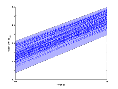
Bounds on the set of consistent parameters, together with sampled consistent parameters, plotted in parallel coordinates.
From the parallel coordinates plot, we observe that there seems to be a correlation in the consistent parameters: from the sampled parameter vectors, either both elements are low, or both are high within the respective intervals. With our choice of 'box shrinkage' as method to approximate the set of consistent parameters, this correlation could not be revealed in the resulting approximation. However, you can redo the above analysis with:
   >>> options.set_exclusion.method = {'bisection'};
   >>> options.plottype = 'bisection - kc';
   >>> [sdpresult, sdpproblem] = parameter_estimation(system, uncertainty, options);
   >>> visualize_uncertainty(sdpresult, samples.p, options);

and indeed such a correlation is clearly visible from the box plots:
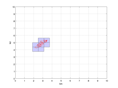
Box plot of approximation to the set of consistent parameters, together with sampled consistent parameters.
Next steps
Congratulations, you have completed the tutorial and should now be familiar with the basic functionality of the bioSDP Toolbox! To dive further in, have a look at the example scripts in the examples directory of the package. For even more details, read the Matlab inline help help <function name> for the toolbox methods which are used in this tutorial or in the examples. And, finally, start working on your models and data!